
Hedge funds struggle with infrequent reporting. Alternative betas offer more timely and accurate performance estimates.
9 min read | Dec 15, 2022
Most hedge funds report returns only with lower frequency, e.g., weekly or monthly. Yet, many market events play out during a few days only. This imposes the risk that one might miss important dynamics when looking at a time series of monthly returns only. In this post we outline how we can utilize “alternative betas” as well as market “betas” to get an estimate of returns with higher frequency.
The Method
We typically view hedge fund returns as a combination of “beta”, which is described by the fund’s co-movement with broad market indices, “alternative beta”, which describe the generation of sophisticated alternative risk premiums that cannot be harvested by holding long market indices alone, and “alpha,” which describes the manager’s ability to generate superior returns. In order to formalize this relation, assume \\( r^i_t \\) describes hedge fund’s \\( i \\) monthly return at time \\( t \\) in excess of the risk free rate. Furthermore assume we can observe \\( N \\) market factors and \\( G \\) alternative risk premia with monthly returns of \\( r^{Mrt, j}_t \\) and \\( r^{alt, j}_t \\), both in excess of the risk free rate. Then the fund returns can be written as:
[1] \\[ r^i_t = \alpha^i_t + \sum_{j=1}^N \beta_{Mrt, j}^i r^{Mrt, j}_t + \sum_{j=1}^G \beta^i_{alt, j} r^{alt, j}_t \\]
Note that \\( \alpha^i_t \\) is hedge fund’s \\( i \\) alpha and time varying as we define it as:
[2] \\[ \alpha^i_t = r^i_t -\left( \sum_{j=1}^N \beta_{Mrt, j}^i r^{Mrt, j}_t + \sum_{j=1}^G \beta^i_{alt, j} r^{alt, j}_t \right) = \alpha^i + \epsilon^i_t \\]
Alpha is thus defined as the hedge fund’s return in month \\(t \\) minus the fraction of the return explained by either beta or alternative premia. This is equivalent to defining alpha as the constant in an OLS regression plus the regression residuals in each month, which is above stated in the last equation.
Circling back to the original question of how to increase the time frequency of hedge fund returns, it is helpful to look more closely at equation [1]. While \\( r^i_t \\) is available in most cases only at lower frequency, e.g., monthly, \\( r^{Mrt, j}t \\) and \\( r^{alt, j}_t \\) can usually be observed at much higher frequency, e.g., weekly, daily, intraday, etc. As a result, we can easily capture the fraction of hedge fund returns \\( i \\) described by “alternative beta” and “beta” at any time frequency where market indices and alternative premia are available. For simplicity, we will focus on daily data in the following. Unlike “alternative beta” and “beta,” the definition of alpha in equation [2] relies on fund returns and is thus tied to the available frequency of fund returns. To bring it down to a daily frequency, we make the simplifying assumption that alpha is generated at a constant rate on each day of a month, which adds up to the observable monthly alpha \\(\alpha^i_t\\). Note that while we assume that this rate is the same for each day within a certain month, the rate can differ for days of different months. Thus, we assume that for each day \\(\tau\\) in month \\(t\\), alpha \\(\alpha^i_\tau\\) can be calculated as follows:
[3] \\[\alpha^i_\tau = \left(1 + \alpha^i_t\right)^\frac{1}{days \; in \; t}-1\\]
where \\[days \; in \; t\\] states the number of trading days in month \\(t\\). We thus can calculate an fund’s daily return estimate as:
[4] \\[\hat{r}^i_\tau = \alpha^i_\tau + \sum^N_{j=1} \beta^i_{Mrt, \; j}r^{Mrt, \; j}_\tau + \sum^G_{j=1}\beta^i_{alt, \; j}r^{alt, \; j}_\tau\\]
Note that this constant definition of alpha and the split into a sum of different contributers introduces an compounding effect which can be easily controlled for by calculating the compounding factor \\(comp_t\\) for each month \\(t\\) and multiplying to \\(\hat{r}^i_\tau\\). We do so by assuming that the compounding effect is constant over time such that:
[5] \\[\prod^{days \; in \; t}_{\tau=1} \left(1+\hat{r}^i_{\tau}comp_t \right) = 1+r^i_t\\]
We solve equation [5] numerically for each month \\(t\\). Having obtained \\(comp_t\\) we can calculate the daily return as:
[6] \\[r^i_\tau = \hat{r}^i_\tau* comp_t\\]
The Method In Action
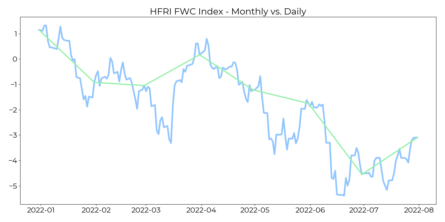
The following chart shows the approach described above applied to the HFRI Fund Weighted Composite Index. In doing so, we estimate equation [1] using the monthly returns of a three-year period and calculate the daily returns according to equations [4]– [6]. We use all RC beta and alternative beta factors as outlined in a pervious post and run a LASSO selection to reduce the number of exogenous variables. The following charts show the daily cumulative returns (blue) and the monthly cumulative returns (green) for the first 7 months of 2022:
(click on the chart below to increase the size)
Besides a pure frequency increase, the above method can also be used to visualize the contribution of alpha, “alternative beta” and “beta”. We do this in the following graph. Here, we look at the HFRI Fund Weighted Composite as well as five strategy-specific HFRI indices. To increase readability, we do not plot the monthly returns but stick to the index daily returns and its three components (as outlined above, it is assumed that alpha has a constant rate within a month):
(click on the chart below to increase the size)
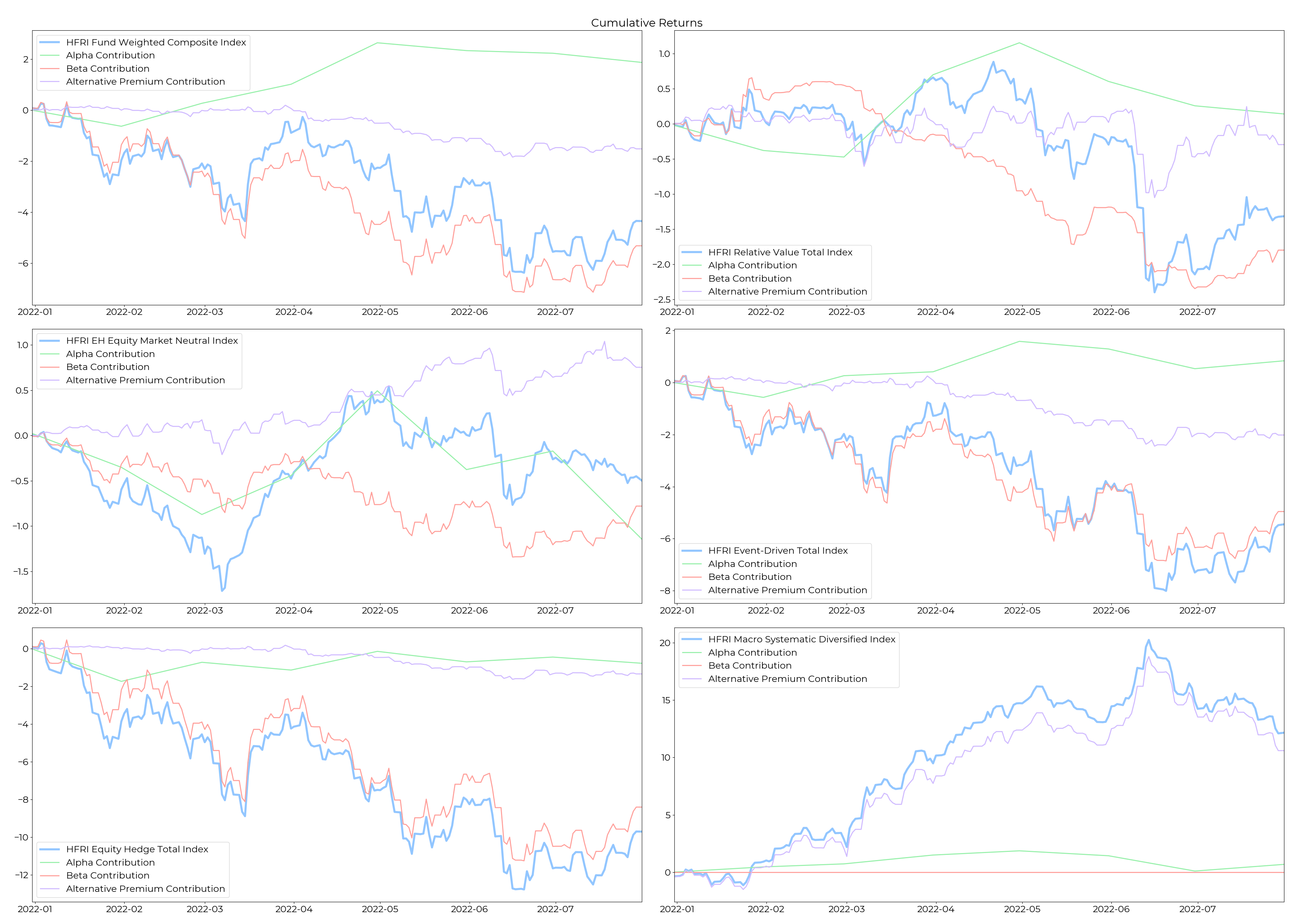
Although all charts contain important information, we focus on only a few observations to highlight the mechanism of the approach. First, let’s look at the decomposition of the HFRI Relative Value Total Index (top right). While the index was slightly down YTD, we can see that the index experienced a significant decline in mid-June, which was very sharp. This decline was mainly due to “alternative beta” as can be seen from the simultaneous decline in the purple line. Furthermore, if we look at the HFRI EH Equity Market Neutral Index (center left), we see a relatively consistent upward movement from March to May with little daily variation, largely due to significant alpha. Finally when looking at the HFRI Macro Systematic Diversified Index, one can see that returns are largely due to alternative beta.
Fit Of The Method
It should be noted that the outlined approach only uses in-sample data. This is not critical, however, as the method does not attempt to predict returns, but rather increases the frequency of monthly returns to daily returns. The cumulative daily returns for a month always match the corresponding observed monthly returns. Nevertheless, it is useful to evaluate the fit of the model to see if the estimated daily returns are potentially close to the true unobservable daily returns. Adj. R2 is the usual candidate for evaluating model fit:
| Index | Adj. R2 | Ido. Vol | Num. Factors |
| HFRI Fund Weighted Composite Index | 88.0 | 0.008 | 3 |
| HFRI Relative Value Total Index | 88.1 | 0.007 | 3 |
| HFRI EH Equity Market Neutral Index | 52.7 | 0.006 | 3 |
| HFRI Event Driven Total Index | 87.9 | 0.010 | 4 |
| HFRI Equity Hedge Total Index | 90.0 | 0.010 | 3 |
| HFRI Macro Systematic Diversified Index | 69.9 | 0.012 | 1 |
Table 1: Replication fit for different HFRI indices. Source: Resonanz Capital
The table above shows that the adjusted R2 for most indices is just below 0.9, with the exception of the HFRI Macro Systematic Diversified Index (0.7) and the HFRI EH Equity Market Neutral Index (0.5). So, in general, the fit is very good. Next, we can look at idiosyncratic volatility, which is the volatility of the regression residuals. The lower the Ido Vol, the lower the volatility of alpha according to equation [2] and the higher the probability that a constant rate of alpha within a month is not an overly unrealistic assumption. In fact, we find very low Ido Vol for all indices, some of them are below 1 basis point. The HFRI EH Equity Market Neutral Index has the lowest Ido Vol overall. So even though the index has a relatively low adjusted R2, it shows a low Ido Vol and thus the model is still reliable.
Conclusion
The utilization of market betas and alternative betas to estimate hedge fund returns at a higher frequency allows for a new perspective on funds’ performance. It enables us to explore beyond the limitation of monthly return data, providing an in-depth understanding of the daily intricacies of fund performance. This development is particularly crucial in contexts where noteworthy market events could have varying impacts within a single month.
Despite potential limitations associated with true alpha funds, which might have minimal exposure to beta and alternative beta factors, this methodology still proves effective. Although there might be some deviation in estimating daily returns for such funds, it’s crucial to note that the approach we’ve designed ensures a rigorous alignment with the verified monthly hedge fund returns, irrespective of the time frame involved.
To sum up, while this method offers a more detailed perspective on hedge fund performance, it’s crucial to understand its limitations. As always, investment decisions should be based on a comprehensive assessment of all available data, including but not limited to higher frequency return analyses.
Resonanz insights in your inbox...
Get the research behind strategies most professional allocators trust, but almost no-one explains.